> ## Documentation Index
> Fetch the complete documentation index at: https://tif1.tracinginsights.com/llms.txt
> Use this file to discover all available pages before exploring further.

# G-G Diagram (Acceleration Envelope)

> Visualize car performance limits with lateral and longitudinal acceleration

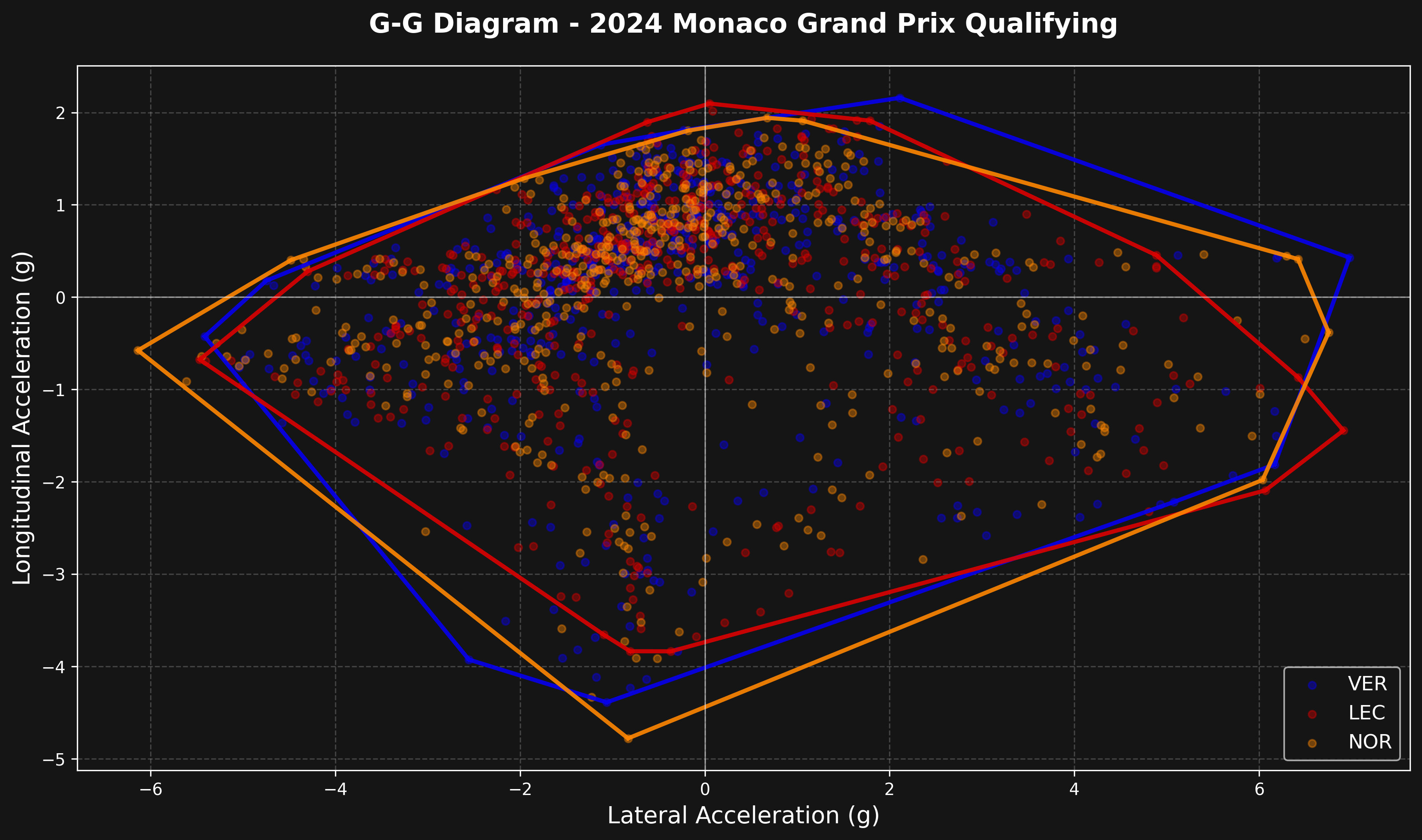
A G-G diagram plots lateral vs longitudinal acceleration, showing the performance envelope of a car. The outer boundary represents the maximum grip available - it's one of the most insightful ways to compare car performance and driver technique.

<img src="https://mintcdn.com/tracinginsightscom/UgQgVDzHEEleARPO/assets/gg_diagram.png?fit=max&auto=format&n=UgQgVDzHEEleARPO&q=85&s=3727f84220bfafa7a11b1a7268e7240f" alt="G-G diagram showing acceleration envelope" width="3570" height="2110" data-path="assets/gg_diagram.png" />

## What is a G-G diagram?

The G-G diagram shows:

* X-axis: Lateral acceleration (cornering forces)
* Y-axis: Longitudinal acceleration (braking/accelerating forces)
* Each point represents a moment in time during the lap
* The outer boundary shows the car's performance limit

## Load session and get telemetry

We'll compare multiple drivers at Monaco Qualifying.

```python theme={"theme":{"light":"github-light","dark":"github-dark"}}
import math
import matplotlib.pyplot as plt
import numpy as np
from scipy.spatial import ConvexHull

import tif1
from tif1.plotting import get_team_color, setup_mpl

# Setup plotting
setup_mpl(color_scheme="fastf1")

# Load session
session = tif1.get_session(2024, "Monaco", "Q")
laps = session.laps

# Select drivers to compare
drivers = ["VER", "LEC", "NOR"]
```

## Compute accelerations

Calculate g-forces from telemetry data using smooth derivatives to reduce noise.

<Note>
  The `smooth_derivative()` function uses a low-noise differentiator algorithm that reduces noise in the acceleration calculations. This is important because raw numerical derivatives amplify noise in the telemetry data, which would create unrealistic spikes in the G-G diagram.
</Note>

```python theme={"theme":{"light":"github-light","dark":"github-dark"}}
def smooth_derivative(t_in, v_in):
    """Compute smooth derivative using low-noise differentiators."""
    t = t_in.copy()
    v = v_in.copy()

    # Transform time to seconds
    try:
        for i in range(0, t.size):
            t.iloc[i] = t.iloc[i].total_seconds()
    except Exception:
        pass

    t = np.array(t)
    v = np.array(v)

    dvdt = np.zeros(t.size)

    # Manually compute boundary points
    dvdt[0] = (v[1] - v[0]) / (t[1] - t[0])
    dvdt[1] = (v[2] - v[0]) / (t[2] - t[0])
    dvdt[2] = (v[3] - v[1]) / (t[3] - t[1])

    n = t.size
    dvdt[n - 1] = (v[n - 1] - v[n - 2]) / (t[n - 1] - t[n - 2])
    dvdt[n - 2] = (v[n - 1] - v[n - 3]) / (t[n - 1] - t[n - 3])
    dvdt[n - 3] = (v[n - 2] - v[n - 4]) / (t[n - 2] - t[n - 4])

    # Compute interior points with smooth method
    c = [5.0 / 32.0, 4.0 / 32.0, 1.0 / 32.0]
    for i in range(3, t.size - 3):
        for j in range(1, 4):
            dvdt[i] += 2 * j * c[j - 1] * (v[i + j] - v[i - j]) / (t[i + j] - t[i - j])

    return dvdt


def truncated_remainder(dividend, divisor):
    """Calculate truncated remainder."""
    divided_number = dividend / divisor
    divided_number = -int(-divided_number) if divided_number < 0 else int(divided_number)
    remainder = dividend - divisor * divided_number
    return remainder


def transform_to_pipi(input_angle):
    """Transform angle to [-pi, pi] range."""
    pi = math.pi
    revolutions = int((input_angle + np.sign(input_angle) * pi) / (2 * pi))
    p1 = truncated_remainder(input_angle + np.sign(input_angle) * pi, 2 * pi)
    p2 = (
        np.sign(
            np.sign(input_angle)
            + 2 * (np.sign(math.fabs((truncated_remainder(input_angle + pi, 2 * pi)) / (2 * pi))) - 1)
        )
        * pi
    )
    output_angle = p1 - p2
    return output_angle, revolutions


def remove_acceleration_outliers(acc):
    """Remove unrealistic acceleration values (> 7.5g)."""
    acc_threshold_g = 7.5
    if math.fabs(acc[0]) > acc_threshold_g:
        acc[0] = 0.0
    for i in range(1, acc.size - 1):
        if math.fabs(acc[i]) > acc_threshold_g:
            acc[i] = acc[i - 1]
    if math.fabs(acc[-1]) > acc_threshold_g:
        acc[-1] = acc[-2]
    return acc


def compute_accelerations(telemetry):
    """Calculate longitudinal and lateral accelerations in g using smooth derivatives."""
    # Longitudinal acceleration from speed change
    v = np.array(telemetry["Speed"]) / 3.6
    lon_acc = smooth_derivative(telemetry["Time"], v) / 9.81

    # Lateral acceleration from track curvature
    dx = smooth_derivative(telemetry["Distance"], telemetry["X"])
    dy = smooth_derivative(telemetry["Distance"], telemetry["Y"])

    # Calculate heading angle
    theta = np.zeros(dx.size)
    theta[0] = math.atan2(dy[0], dx[0])
    for i in range(0, dx.size):
        theta[i] = theta[i - 1] + transform_to_pipi(math.atan2(dy[i], dx[i]) - theta[i - 1])[0]

    # Curvature is rate of change of heading
    kappa = smooth_derivative(telemetry["Distance"], theta)
    lat_acc = v * v * kappa / 9.81

    # Remove outliers
    lon_acc = remove_acceleration_outliers(lon_acc)
    lat_acc = remove_acceleration_outliers(lat_acc)

    return lon_acc, lat_acc
```

## Create G-G diagram

Plot acceleration data with performance envelope using convex hull.

<Note>
  The performance envelope is computed using `scipy.spatial.ConvexHull`, which finds the smallest convex polygon that contains all acceleration points. This accurately represents the car's performance limits across all directions of acceleration.
</Note>

```python theme={"theme":{"light":"github-light","dark":"github-dark"}}
fig, ax = plt.subplots(figsize=(12, 12))

for driver in drivers:
    try:
        # Get fastest lap telemetry
        driver_lap = laps.pick_driver(driver).pick_fastest()
        telemetry = driver_lap.get_telemetry().add_distance()

        # Compute accelerations
        lon_acc, lat_acc = compute_accelerations(telemetry)

        # Get team color
        try:
            team = driver_lap["Team"] if "Team" in driver_lap.index else None
            color = get_team_color(team) if team else None
        except Exception:
            color = None

        if color is None:
            # Fallback colors
            color_map = {"VER": "#0600ef", "LEC": "#dc0000", "NOR": "#ff8700"}
            color = color_map.get(driver, "#ffffff")

        # Plot scatter points
        ax.scatter(
            lat_acc,
            lon_acc,
            s=20,
            alpha=0.4,
            color=color,
            label=driver,
        )

        # Draw performance envelope using ConvexHull
        points = np.column_stack([lat_acc, lon_acc])
        points = points[~np.isnan(points).any(axis=1)]

        if len(points) > 3:
            try:
                hull = ConvexHull(points)
                # Plot the convex hull edges
                for simplex in hull.simplices:
                    ax.plot(
                        points[simplex, 0],
                        points[simplex, 1],
                        color=color,
                        linewidth=2.5,
                        alpha=0.9,
                    )
            except Exception as hull_error:
                print(f"Warning: Could not compute convex hull for {driver}: {hull_error}")
                continue

    except Exception as e:
        print(f"Warning: Could not process {driver}: {e}")
        continue

# Styling
ax.set_xlabel("Lateral Acceleration (g)", fontsize=14)
ax.set_ylabel("Longitudinal Acceleration (g)", fontsize=14)
ax.set_title(
    f"G-G Diagram - {session.event.year} {session.event['EventName']} {session.name}",
    fontsize=16,
    fontweight="bold",
    pad=20,
)

# Add grid and axis lines
ax.grid(True, alpha=0.3, linestyle="--")
ax.axhline(0, color="white", linestyle="-", alpha=0.5, linewidth=0.8)
ax.axvline(0, color="white", linestyle="-", alpha=0.5, linewidth=0.8)

# Set equal aspect ratio for proper g-force visualization
ax.set_aspect("equal")

# Legend
ax.legend(loc="lower right", fontsize=12)

plt.tight_layout()
plt.show()
```

## Reading the diagram

Key insights from a G-G diagram:

* **Top of envelope (positive Y):** Maximum acceleration
* **Bottom of envelope (negative Y):** Maximum braking
* **Left/right edges (X):** Maximum cornering forces
* **Corners of envelope:** Combined braking/acceleration + cornering
* **Wider envelope:** More grip available
* **Rounder envelope:** Better balanced car

## Comparing drivers

Look for:

* **Envelope size:** Larger = more grip being used
* **Envelope shape:** Asymmetry shows car balance issues
* **Point density:** Where drivers spend most time
* **Peak values:** Maximum g-forces achieved

## Track characteristics

Different tracks produce different shapes:

* **Monaco:** Smaller envelope, lower speeds, less extreme forces
* **Monza:** Larger longitudinal values (high-speed braking)
* **Silverstone:** Large lateral values (high-speed corners)

The G-G diagram is a powerful tool for understanding car performance limits and how drivers extract maximum grip from the car.